FDM heat equation of isolated rod with dynamic end temparatures

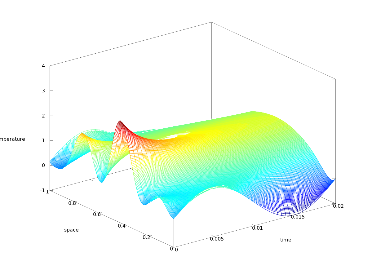
To test my understanding of the FDM method I made a simple implementation of the Crank-Nickelson method applied on the heat equation. The physical intepretation is this: You have a perfectly insulated rod of length \(l\). At time \(t_0\) you know the temperature distribution in the rod, \(f(x)\). You also know that each end of the rod will have a temperature that is a function of time, \(g_0(t)\) and \(g_1(t)\). Given this information, what will the temperature in the rod be at an arbitraray time \(t\) and position \(x\)? This is what the heat equation tells you, the problem, as usual with partial differential equations is that you can't always solve them explicitly. This is where numerical techniques comes to play and saves the day. Below is the result of a numerical simulation of such a senario. For simplicity the rods length is \(1\).

\[ f(x) = (2+2\sin(6 \pi x)) (1-|2(x-1)|), 0 \leq x \leq1 \] \[ g_0(x) = g_1(x) = \sin(t), 0 \leq t \]

This gives rise to the following solution:

Here is the Octave code that calculates this plot, quite simple and self explanetory:

M = 401; % number of space nodes
h = 1/(M+1); % space step size

T = 40000;  % number of timesteps
t = 0.0000005; % time step size

%U0 = 1-abs(linspace(-1,1,M)); % initial data
U0 = (2+2*sin(linspace(0,6*pi,M))).*(1-abs(linspace(-1,1,M))); % initial data
G1 = sin(linspace(0,2*pi,T));
GM = G1;

r = t/h^2;

U = zeros(M,T);
U(:,1) = U0;

n = M;
e = ones(n,1);
A = spdiags([e, -2*e, e], -1:1, n, n);

lkern = eye(M) + (r/2)*A;
rkern = eye(M) - (r/2)*A;

%for y=1:100
  U(:,1) = U0;
  for i=1:T-1
    U(:,i+1) = rkern\(lkern*U(:,i));
    U(1,i+1) = G1(i+1);
    U(M,i+1) = GM(i+1);
  end
%end

downscale = 1000;

Y = zeros(M,T/downscale);
for i=1:T/downscale;
  Y(:,i) = U(:,downscale*i);
end

tx = linspace(0,1,M);
tt = linspace(0,t*T,T/downscale);
hold off
mesh(tt,tx,Y);
%contour(U)
ylabel('space');
xlabel('time');